In part 1 I wrote about building an application that is, effectively, the love child of a flow chart and a to do list, and how that presented the problem of modeling DAGs in SQL. I went on to explain how the closure table pattern could be used to model trees. This post will close the loop by showing how the closure table pattern can be extended to support not only trees but DAGs as well.
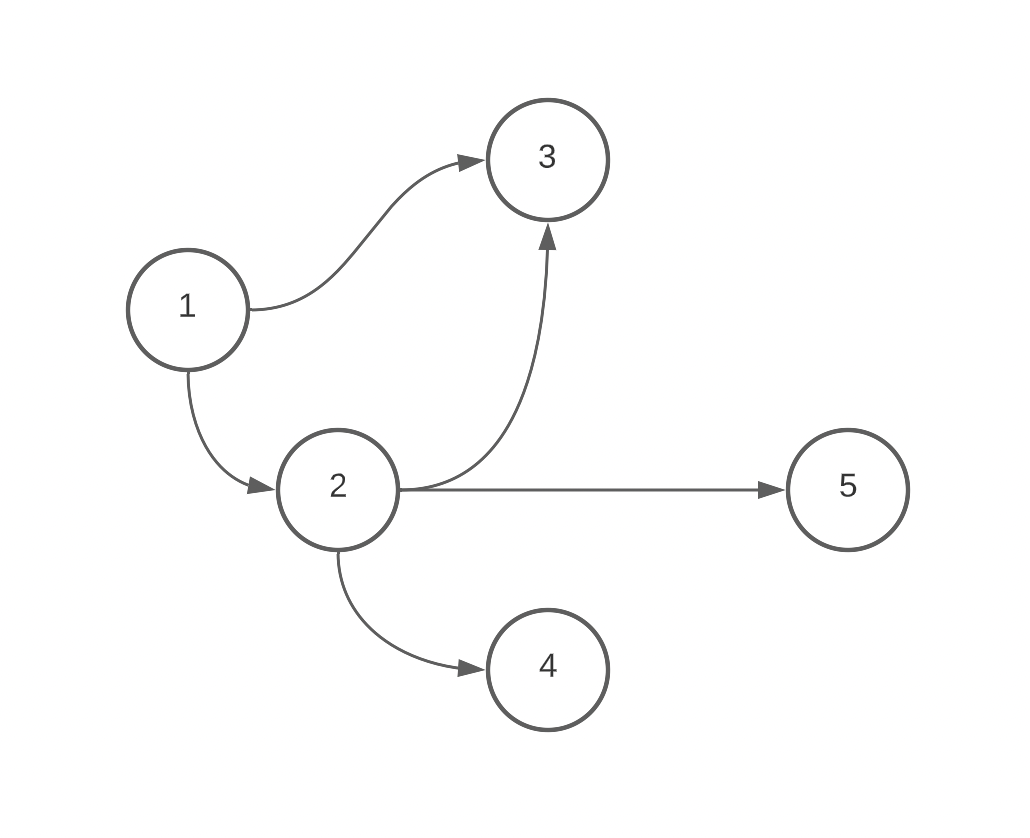
(An example of a DAG)
Problems presented by transitioning from a tree to a DAG
In part 1, there were several assumptions that allowed the closure table pattern and the associated queries to work so smoothly:
- All new connections were happening between childless nodes and brand new nodes.
- There was only ever a single path from parent to child (even if that path was represented by many records).
- Subtrees were always deleted in their entirety rather than being maintained as separate entities.
With my DAG-based to do list application, all of these nice and tidy assumptions had to be thrown out. Instead, I wanted users to be able to:
- Make connections at any level of the graph for both new and existing nodes.
- Have one node be the parent of another through multiple paths. For example, it should be possible to have
1 -> 3and1 -> 2 -> 3at the same time (like in the image above). - Separate a portion of the graph and have it exist on its own.
With those problems in mind, let’s lay out the data model.
Updating the data model
As a reminder, here’s the data model from part 1:
CREATE TABLE nodes (
  id SERIAL PRIMARY KEY
);

CREATE TABLE edges (
  source INT REFERENCES nodes (id) ON DELETE CASCADE,
  destination INT REFERENCES nodes (id) ON DELETE CASCADE,
  PRIMARY KEY (source, destination)
);
In order to support our new use cases above, we need to add two fields, depth and count, to our edges table and include depth in our primary key:
CREATE TABLE edges (
  source INT REFERENCES nodes (id) ON DELETE CASCADE,
  destination INT REFERENCES nodes (id) ON DELETE CASCADE,
  depth INT NOT NULL DEFAULT 0,
  count INT NOT NULL DEFAULT 1,
  PRIMARY KEY (source, destination, depth)
);
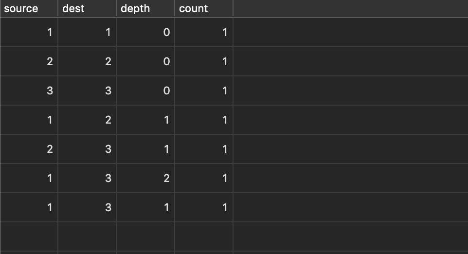
Let’s start by explaining depth. depth represents how many edges are between a given set of connected nodes. Knowing the depth of an edge allows us to correctly manage situations in which multiple edges have the same source and destination, but there is more than one configuration of intermediary nodes. This is the case above of having both 1 -> 3 and 1 -> 2 -> 3 at the same time. With depth added to the data model, the above would be represented like this in our edges table:
Although depth plays a key role in supporting count (more on this in a second), the most direct use it has is in allowing us to correctly remove connections in situations like the one above. Deletions of edges work like so:
CREATE FUNCTION delete_edge (delete_source int, delete_destination int) RETURNS VOID
AS $$
WITH selected_edges AS (
	SELECT l.source as source, r.destination as destination, l.depth + r.depth + (CASE WHEN delete_source = delete_destination THEN 0 ELSE 1 END) as depth FROM (
		(SELECT * FROM edges WHERE destination = delete_source) l
		CROSS JOIN
		(SELECT * FROM edges WHERE source = delete_destination) r
	)
), updated AS (
	UPDATE edges SET count = count - 1
	WHERE (source, destination, depth) IN (
		SELECT source, destination, depth FROM selected_edges
	) AND count > 1
) DELETE FROM edges WHERE (source, destination, depth) IN (SELECT source, destination, depth FROM selected_edges) AND count = 1;
$$ LANGUAGE SQL;
In addition to using depth to properly select which edges to update or delete, we’re also now doing a cross join on all the children of our destination and all the parents of our source. This is a major change from the closure table pattern queries in part 1, and what necessitates the added complexity is the fact that we’re no longer working at the childless tip of a tree. Instead, we need to make sure that we create the cross references as we connect, for example, the tip of one graph with the head of another so that we can continue to make nice and simple SELECT queries like:
SELECT destination FROM edges WHERE source = 2;
On to count. count is necessary for situations in which two nodes are connected multiple times over the same distance. The simplest example begins below:
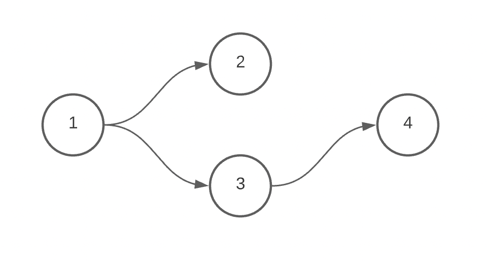
With count, we can properly represent a situation in which we’d also like to connect node 2 to node 4. In that case, we first check to see if a connection to 1 and 4 already exists. It does (through 3), so instead of inserting a new edge with a source of 1 and a destination of 4, we increment the count of the existing edge. The creation of the edge with 2 as the source and 4 as the destination proceeds like normal. This logic can be succinctly summarized as ‘insert or increment’ and its corollary when removing edges is ‘decrement or delete’.
The insert query looks like this:
CREATE FUNCTION insert_edge (insert_source int, insert_destination int) RETURNS edges
AS $$
WITH cycle_check AS (
	SELECT * FROM edges WHERE destination = insert_source AND source = insert_destination
), cross_inserts AS (
	SELECT l.source as source, r.destination as destination, l.depth + r.depth + 1 as depth FROM (
		(
			SELECT * FROM edges WHERE destination = insert_source
			AND NOT EXISTS (SELECT * FROM cycle_check)
		) l
		CROSS JOIN
		(
			SELECT * FROM edges WHERE source = insert_destination
			AND NOT EXISTS (SELECT * FROM cycle_check)
		) r
	)
) INSERT INTO edges (source, destination, depth)
	SELECT source, destination, depth FROM cross_inserts
	ON CONFLICT ON CONSTRAINT edges_pkey
	DO UPDATE SET count = EXCLUDED.count + 1
	RETURNING *
$$ LANGUAGE SQL;
(One thing worth noting that’s different from Part 1 with this edge creation query is that we’re no longer creating a loopback record when connecting edges. Instead, we create the loopback when the node is initially created. This avoids the problem of maintaining the loopback’s proper count in cases where a node has multiple parents.)
After running that query, inputting 2 and 4 for source and destination, our edges table contains:
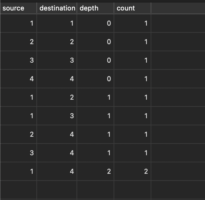
Note that the 9th record, which shows the connection of node 1 to node 4 has a depth of 2 (since it’s not a direct connection) and a count of 2, since 1 and 4 are connected both via 2 and 3.
Also, recall that we added depth to the primary key. The primary key is violated not just because another edge has the same source and destination but also the same depth. In other words, depth being in the primary key is part of the trigger for incrementing on an existing record rather than inserting a new record. This helps to keep proper counts in a situation in which a node is connected to another node multiple times. For example, 1 -> 2 -> 3 -> 4, 1 -> 2 -> 4, 1 -> 4 all have different depths and therefore their counts are kept separate when, say, 1 -> 3 -> 4 is added next.
Conclusion
I’ve yet to test this approach at scale, but for the sake of my personal project I’m happy with how straightforward it was to implement. The Closure Table pattern is the foundation, and with the addition of couple extra fields a variety of complex use cases can be supported. This solution seems especially useful in situations in which a relational DB is already set up as a part of an existing project and it isn’t feasible or desirable to start futzing around with a graph-specific DB.