This past year I built an app that allows users to create and manage their to do list as a kind of flow chart. The nodes were tasks, the edges dependencies (‘get groceries’ must occur before ‘make dinner’, etc.), and creating loops of any kind wasn’t allowed (there are other apps for making and sustaining good habits). In other words, the app was a specific application of a Directed Acyclic Graph (DAG).
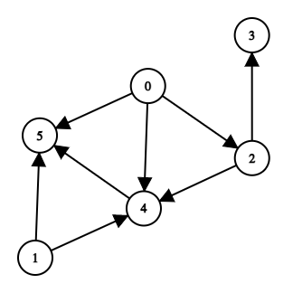
An example of a DAG
The app provides several interesting engineering problems, but the one I’m going to focus on in the following two posts is the database layer, specifically using Postgres.
Thankfully, there’s no shortage of prior art on this subject. After doing some research, I decided to use was the Closure Table pattern. The rest of this post will explain what that is and part two will explain how to adapt it to support DAGs.
The Closure Table Pattern
The Closure Table Pattern is based on the idea that we can make a space tradeoff for quicker access and a simpler set of queries. The data model for this pattern looks like this:
CREATE TABLE nodes (
  id SERIAL PRIMARY KEY
);

CREATE TABLE edges (
  source INT REFERENCES nodes (id) ON DELETE CASCADE,
  dest INT REFERENCES nodes (id) ON DELETE CASCADE,
  PRIMARY KEY (source, dest)
);
Nothing fancy so far. The secret sauce is in what records are created when two nodes are connected. For example, say we have the following structure:
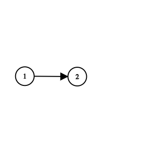
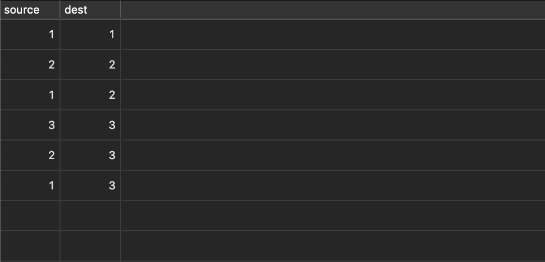
In our database, that would look like the following:
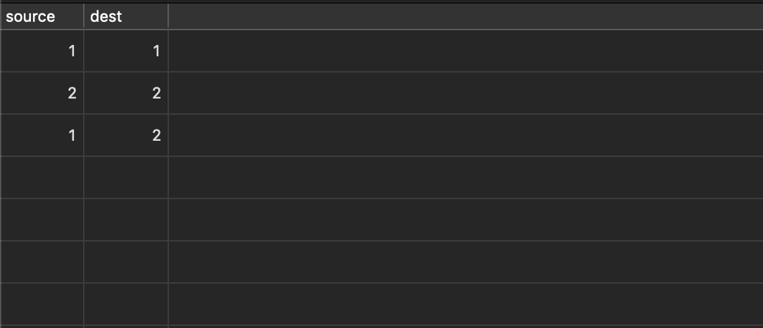
Note the extra records in which the nodes connect to themselves (what I call ‘loopback’ edges). I’ll come back to why these are useful in a second. Now, we create a new node and connect node 2 to it like so:
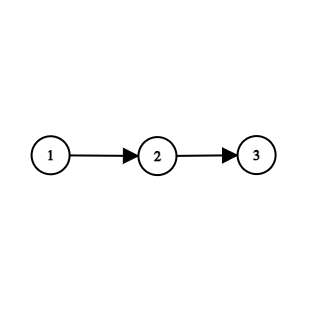
Now, not only do we create a new edge with 2 as its source and 3 as its destination, but we also create another edge with 1 as its source and 3 as its destination, as well as a new loopback edge for node 3. The result looks like this:
The query itself is:
INSERT INTO edges (source, dest)
SELECT source, 3 FROM edges
WHERE dest = 2
UNION ALL SELECT 3, 3; -- This creates the new loopback
Note that without node 2’s loopback edge, we wouldn’t’ve actually connected 2 & 3. This is the primary reason why the loopback edges are useful.
The beauty of this approach is that by making a space trade off (creating potentially many more edge records, depending on how large and deep a given tree is), we are able to much more quickly and easily make a number of queries. For example, give me all the children of a node:
SELECT dest FROM edges WHERE source = 1;
Pretty simple, right?
Or, give me all of the parents of a node:
SELECT source FROM edges WHERE dest = 3;
Deletions are even more straightforward:
DELETE FROM edges WHERE dest = 4;
Finally, deleting a subtree:
DELETE FROM edges
WHERE dest IN (
	SELECT dest FROM edges
	WHERE source = 2
);
As you can see, all of these queries are nice and succinct, and the mental model that undergirds them them isn’t too complex either. It’s a fantastic pattern if you’re working with a tree, but if have a non-hierarchical structure (like our aforementioned DAG) then you’re going to run into problems. In the next post, I’ll cover what some of those problems are and how we can adapt the closure table pattern to solve them.
Additional Reading:
- From what I could glean, Joe Celko was the first person to write about this pattern in his 1998 (!) book ‘SQL for Smarties’
- Bill Karwin has an an excellent explanation of the closure table pattern here
- If you’re looking for other ways of representing hierarchical data in SQL, look no further than this great wiki